Abstractive Summarization with HuggingFace pre-trained models
Text summarization is a well explored area in NLP. As shown in Figure 1, the field of text summarization can be split based on input document type, output type and purpose. Regarding output type, text summarization dissects into extractive and abstractive methods.
• Extractive: In the Extractive methods, a summarizer tries to find and combine the most significant sentences of the corpus to form a summary. There are some techniques to identify the principal sentences and measure their importance such as Topic Representation, and Indicator Representation.
• Abstractive: Abstractive Text Summarization (ATS) is the process of finding the most essential meaning of a text and rewriting them in a summary. The resulting summary is an interpretation of the source. Abstractive summarization is closer to what a human usually does. He conceives the text, compares it with his memory and related in-formation, and then re-create its core in a brief text. That is why the abstractive summarization is more challenging than the extractive method, as the model should break the source corpus apart to the very tokens and regenerate the target sentences. Achieving meaningful and grammatically correct sentences in the summaries is a big deal that demands highly precise and sophisticated models.
In this tutorial, we use HuggingFace‘s transformers library in Python to perform abstractive text summarization on any text we want. The Transformer in NLP is a novel architecture that aims to solve sequence-to-sequence tasks while handling long-range dependencies with ease.
The reason why we chose HuggingFace’s Transformers as it provides us with thousands of pretrained models not just for text summarization, but for a wide variety of NLP tasks, such as text classification, question answering, machine translation, text generation and more.
All the documentation for the transformers library can be found on this website: https://huggingface.co/transformers/
For more information on how transformers are built, we recommend reading the seminar paper ” Attention Is All You Need”.
For usage examples or fine-tuning you can check hugging face community notebook or official notebooks through these links:
- official: https://huggingface.co/transformers/notebooks.html
- community: https://huggingface.co/transformers/v3.0.2/notebooks.html
To install transformers, you can simply run:
!pip install transformers
Then, We need to importing needed dependencies
from transformers import pipeline
Pipeline API
The most straightforward way to use models in transformers is using the pipeline API. The Pipeline are high-level objects which automatically handle tokenization, running your data through a transformers model and outputting the result in a structured object.
In the summarization pipline, the default model is the BART model, which is trained on the CNN/Daily Mail News Dataset.
# Initialize the HuggingFace summarization pipeline
summarizer = pipeline("summarization")

# Open and read the article
TEXT = """
Equitable access to safe and effective vaccines is critical to ending the COVID-19 pandemic, so it is hugely encouraging to see so many vaccines proving and going into development. WHO is working tirelessly with partners to develop, manufacture and deploy safe and effective vaccines.

Safe and effective vaccines are a game-changing tool: but for the foreseeable future we must continue wearing masks, cleaning our hands, ensuring good ventilation indoors, physically distancing and avoiding crowds.

Being vaccinated does not mean that we can throw caution to the wind and put ourselves and others at risk, particularly because research is still ongoing into how much vaccines protect not only against disease but also against infection and transmission.

See WHO’s landscape of COVID-19 vaccine candidates for the latest information on vaccines in clinical and pre-clinical development, generally updated twice a week. WHO’s COVID-19 dashboard, updated daily, also features the number of vaccine doses administered globally.

But it’s not vaccines that will stop the pandemic, it’s vaccination. We must ensure fair and equitable access to vaccines, and ensure every country receives them and can roll them out to protect their people, starting with the most vulnerable.
"""

#run the model
summarized = summarizer(TEXT, min_length=25, max_length=50)

# Print summarized text
print(summarized)
Note that the first time you execute this, it make take a while to download the model architecture and the weights, as well as tokenizer configuration. we declared the min_length and the max_length we want the summarization output to be (this is optional).
The generated summary is:
[{‘summary_text’: ‘ WHO is working tirelessly with partners to develop, manufacture and deploy safe and effective vaccines . We must continue wearing masks, cleaning our hands, ensuring good ventilation indoors, physically distancing and avoiding crowds .’}]
If you want to chnge the model and use the t5 model (e.g. t5-base), which is trained on the c4 Common Crawl web corpus, then change the following statements.
Note that the T5 comes with 3 versions in this library, t5-small, which is a smaller version of t5-base, and t5-large that is larger and more accurate than the others
 #setting the pipeline
summarizer = pipeline("summarization", model="t5-base", tokenizer="t5-base", framework="tf")
#run the model
summarized = summarizer(TEXT, min_length=25, max_length=50)

# Print summarized text
print(summarized)
The second summary is as follows:
[{‘summary_text’: ‘WHO is working tirelessly with partners to develop, manufacture and deploy safe and effective vaccines . but for the foreseeable future we must continue wearing masks, cleaning our hands, ensuring good ventilation indoors, physically distancing’}]
For both models, the generated results illustrate that it works really well, which is really impressive!
I hope you enjoyed the tutorial. To download the notebook click here.

Easy tutorial on Spark SQL and DataFrames
In this tutorial, you will learn how to load a DataFrame and perform basic operations on DataFrames with both API and SQL.
I’m using colab to run the code.
First, we need to To download the required tools
!apt-get install openjdk-8-jdk-headless -qq > /dev/null
!wget -q https://downloads.apache.org/spark/spark-3.1.1/spark-3.1.1-bin-hadoop2.7.tgz
!tar -xvf spark-3.1.1-bin-hadoop2.7.tgz
!pip install -q findspark
Then, add this statement to tell your bash where to find spark. To do so, configure your $PATH variables by adding the following lines
import os
os.environ["JAVA_HOME"] = "/usr/lib/jvm/java-8-openjdk-amd64"
os.environ["SPARK_HOME"] = "/content/spark-3.1.1-bin-hadoop2.7"
Start a spark session
import findspark
findspark.init()
from pyspark.sql import SparkSession
spark = SparkSession.builder.master("local[*]").getOrCreate()
Manipulating dataframes
We need first to import the data file. There are different ways to import a file (from drive, from an URL, or from your local hard disk). Files.upload will upload a file from your hard disk, this is not# recommended for very large files (the example is based on the movielens csv file)
from google.colab import filesfiles.upload()
data = spark.read.format("csv")\
.option("delimiter", ",")\
.option("header", True)\
.load("ratings.csv")
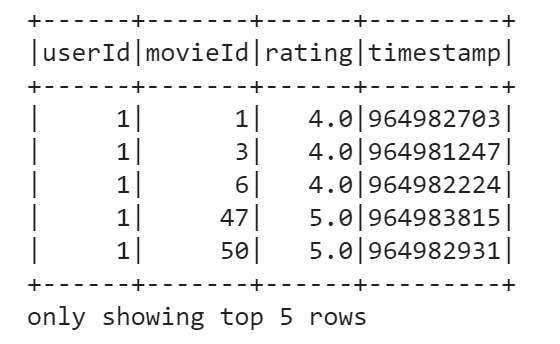
data.show(5)
print((data.count(), len(data.columns)))

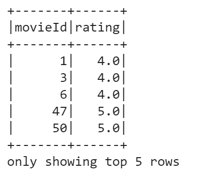
To take a glance at the data, we use the show() method. For instance, we can display first five rows:
data.select("movieId", "rating").show(5)
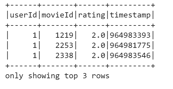
You can also filter the DataFrame based on some condition. Say, we want to choose movies with ratings lower than 3.0. To do this, run the following:
data.filter(data['rating'] < 3.0).show(3)
Another useful operation to perform on a DataFrame is grouping by some field. Let’s group our DataFrame by rating, check counts for each rating, and finally order the resulting counts by rating.
data.groupBy(data['rating']).count().orderBy('rating').show()
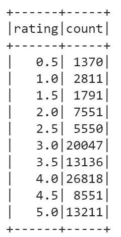
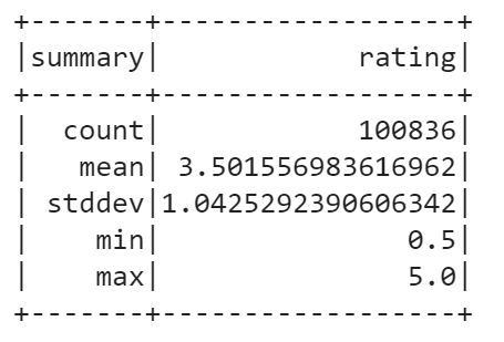
You can also calculate basic statistics for a DataFrame using describe() method. It includes min, max, mean, standard deviation, and count for numeric columns. You may specify columns or calculate overall statistics for a DataFrame. In our case, only rating column is suitable for statistics calculation.
data.describe("rating").show()
Using SQL API
#Now, we will use SQL to query the data. To begin with, we need to register a DataFrame as a temp view with the next command:
data.createOrReplaceTempView("ratings")
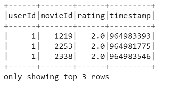
Let’s make the same filtering as before — we’ll select only movies with ratings lower than 3 using SQL:
spark.sql("select * from ratings where rating < 3").show(3)
You can download the code of this tutorial from this link

K-Nearest Neighbors Algorithm with Scikit-Learn
K Nearest Neighbor(KNN) is a very simple, easy to understand, supervised machine learning algorithms. KNN classifier classifies new data in a particular class based on a similarity measure
How does KNN works
A new observation is classified by a majority of its neighbors If K=1, then the class is simply assigned to the class of its nearest neighbor
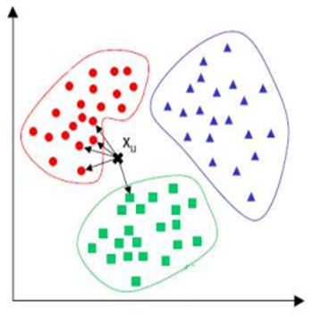
Requires three things
- The set of stored records
- Distance Metric to compute distance between records (for example the Euclidean distance)
- The value of k, the number of nearest neighbors to retrieve
To classify an unknown record:
- Compute distance to other training records
- Identify k nearest neighbors
- Use class labels of nearest neighbors to determine the class label of unknown record (e.g., by taking majority vote)
KNN implementation with Scikit-Learn
Importing Libraries
import numpy as np import matplotlib.pyplot as plt import pandas as pdImporting the iris dataset.
url= "https://archive.ics.uci.edu/ml/machine-learning-databases/iris/iris.data"
names = ['sepal-length', 'sepal-width', 'petal-length', 'petal-width', 'Class']

# Read dataset to pandas dataframe
dataset = pd.read_csv(url, names=names)
Let’s display the five first records. Each observation represents one flower (class value) and 4 columns represents 4 measurements
dataset.head()

The next step is to split our dataset into its attributes and labels
 X = dataset.iloc[:, :-1].values
y = dataset.iloc[:, 4].values
Split the data into training and testing sets
To evaluate the model performance we need to divide the dataset into a training set and a test set. This way our algorithm is tested on un-seen data, as it would be in a production application.
Let’s split dataset by using function train_test_split(). You need to pass 3 parameters features, target, and test_set size.
from sklearn.model_selection import train_test_split
X_train, X_test, y_train, y_test = train_test_split(X, y, test_size=0.20)
Data standardization
As the KNN is based on calculation distance measures, it’s better to standardize the data
from sklearn.preprocessing import StandardScaler
scaler = StandardScaler()
scaler.fit(X_train)

X_train = scaler.transform(X_train)
X_test = scaler.transform(X_test)
Runnin the training and prediction
Let’s build KNN classifier model for k=5.
from sklearn.neighbors import KNeighborsClassifier
classifier = KNeighborsClassifier(n_neighbors=5)
classifier.fit(X_train, y_train)
y_pred = classifier.predict(X_test)
Model Evaluation
There are different measures to evaluate the performance of a classification algorithm as the accuracy, confusion matrix, precision, recall and f1 score. Let’s estimate, how accurately the classifier can predict the type of the flowers. Accuracy is the most intuitive performance measure and it is simply a ratio of correctly predicted observation to the total observations. Accuracy can be computed by comparing actual test set values and predicted values
#Import scikit-learn metrics module for accuracy calculation
from sklearn import metrics
# Model Accuracy, how often is the classifier correct?
print("Accuracy:",metrics.accuracy_score(y_test, y_pred))

Let’s fit and test the model for different values for K (from 1 to 40) using a for loop and record the KNN’s testing accuracy in a list variable (error).
error = []

# Calculating error for K values between 1 and 40
for i in range(1, 40):
    classifier = KNeighborsClassifier(n_neighbors=i)
    classifier.fit(X_train, y_train)
    pred_i = classifier.predict(X_test)
    error.append(metrics.accuracy_score(y_test, pred_i))
Plot the relationship between the values of K and the corresponding testing accuracy using the matplotlib library. As we can see there is a raise and fall in the accuracy
 from matplotlib import pyplot as plt
plt.plot(error)
plt.show()
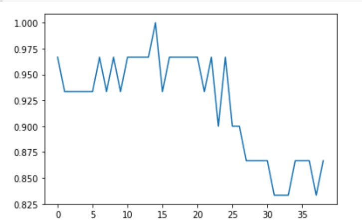
In KNN, finding the value of k is not easy. A small value of k means that noise will have a higher influence on the result and a large value make it computationally expensive. Some researchers recommand to set k=sqrt(n), where n is the dataset size.
You probably got different results from what you see here. This is because dataset splitting is random by default. The result differs each time you run the function. However, this often isn’t what you want.
Sometimes, to make your tests reproducible, you need a random split with the same output for each function call. You can do that with the parameter random_state. The value of random_state isn’t important—it can be any non-negative integer. You could use an instance of numpy.random.RandomState instead, but that is a more complex approach.
X_train, X_test, y_train, y_test= train_test_split(X, y, test_size=0.20,random_state=4)

Data preprocessing key steps
Data preprocessing is a technique that is used to transform raw data into an understandable format. Raw data often contains numerous errors (lacking attribute values or certain attributes or only containing aggregate data) and lacks consistency (containing discrepancies in the code) and completeness. This is where data preprocessing comes into the picture and provides a proven method of resolving such issues.
Steps involved in Data Preprocessing in Machine Learning
- Importing necessary libraries.
- Importing the data-set.
- Checking and handling the missing values.
- Encoding Categorical Data.
- Feature Scaling.
Importing necessary libraries
Python has a list of amazing libraries and modules which help us in the data preprocessing process. Therefore in order to implement data preprocessing the first and foremost step is to import the necessary/required libraries. The libraries that we will be using in this tutorial are: NumPy NumPy is a Python library that allows you to perform numerical calculations. Think about linear algebra in school (or university) – NumPy is the Python library for it. It’s about matrices and vectors – and doing operations on top of them. At the heart of NumPy is a basic data type, called NumPy array. The NumPy API can be referenced here.
Pandas The Pandas library is the fundamental high-level building block for performing practical and real-world data analysis in Python. The Pandas library will not only allow us to import the data sets but also create the matrix of features and the dependent variable vector. The panda API can be referenced here.
Matplotlib The Matplotlib library allows us to plot some awesome charts which is a major requirement in Machine Learning.
import numpy as np
import pandas as pd
import matplotlib.pyplot as plt
Importing The Dataset and exploring the data
Once we have successfully imported all the required libraries, we then need to import the required dataset. For this purpose, we will be using the pandas library.
Let’s read the data (using read_csv), and take a look at the first 5 lines using the head method:
from google.colab import files
uploaded = files.upload()
dataset = pd.read_csv('data.csv')
dataset.head()
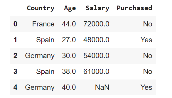
Let’s have a look at data dimensionality, feature names, and feature types.
print(dataset.shape)

From the output, we can see that the table contains 10 rows and 4 columns.
Now let’s try printing out column names using columns:
print(dataset.columns)

We can use the info() method to output some general information about the dataframe:
print(dataset.info())
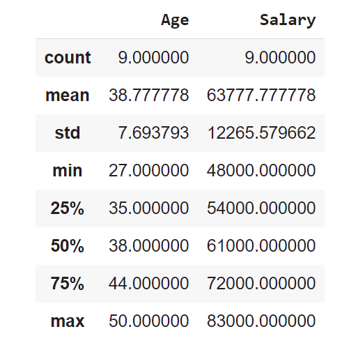
The describe method shows basic statistical characteristics of each numerical feature (int64 and float64 types): number of non-missing values, mean, standard deviation, range, median, 0.25 and 0.75 quartiles.
dataset.describe()
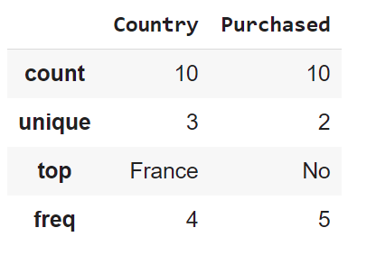
In order to see statistics on non-numerical features, one has to explicitly indicate data types of interest in the include parameter.
dataset.describe(include=['object', 'bool'])
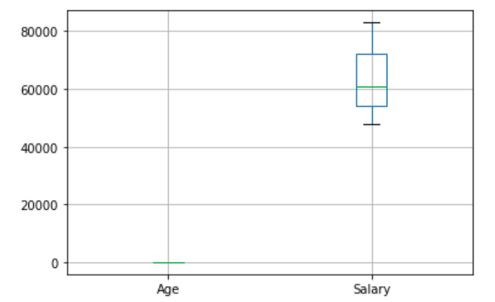
To get more statistic measures on numerical feature we can use the whisker plot. The box extends from the Q1 to Q3 quartile values of the data, with a line at the median (Q2). The whiskers extend from the edges of box to show the range of the data. By default, they extend no more than 1.5 * IQR (IQR = Q3 – Q1) from the edges of the box, ending at the farthest data point within that interval. Outliers are plotted as separate dots.
boxplot = dataset.boxplot()
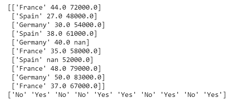
The matrix of features is used to describe the list of columns containing the independent variables to be processed and includes all lines in the given dataset. The target variable vector used to define the list of dependent variables in the existing dataset. iloc is an indexer for the Pandas Dataframe that is used to select rows and columns by their location/position/index.
x = dataset.iloc[:,:-1].values
y = dataset.iloc[:,-1].values
print(x)
print(y)
Handling The Missing Values
While dealing with datasets, we often encounter missing values which might lead to incorrect deductions. Thus it is very important to handle missing values.
There are couple of ways in which we can handle the missing data.
Method 1: Delete The Particular Row Containing Null Value Drop the rows where at least one element is missing:
dataset.dropna(inplace=”true”)
This method is advised only when there are enough samples in the data set. One has to make sure that after we have deleted the data, there is no addition of bias. Removing the data will lead to loss of information which will not give the expected results while predicting the output.
Method 2 Method 2: Replacing The Missing Value With The Mean, Mode, or Median This strategy is best suited for features that have numeric data. We can simply calculate either of the mean, median, or mode of the feature and then replace the missing values with the calculated value. In our case, we will be calculating the mean to replace the missing values. Replacing the missing data with one of the above three approximations is also known as leaking the data while training.
➥ To deal with the missing values we need the help of the SimpleImputer class of the scikit-learn library.
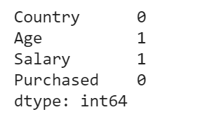
Let’s check how many missing values do we have
dataset.isnull().sum()
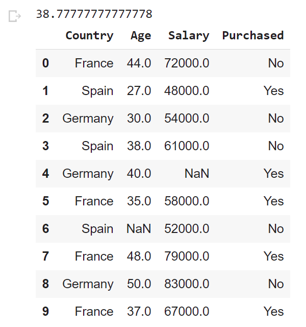
Before replacing the missing values by the mean, let’s display the mean of ages
print(dataset['Age'].mean())
dataset
from sklearn.impute import SimpleImputer
imputer = SimpleImputer(missing_values=np.nan, strategy='mean')
imputer.fit(x[:, 1:3])
x[:, 1:3] = imputer.transform(x[:, 1:3])
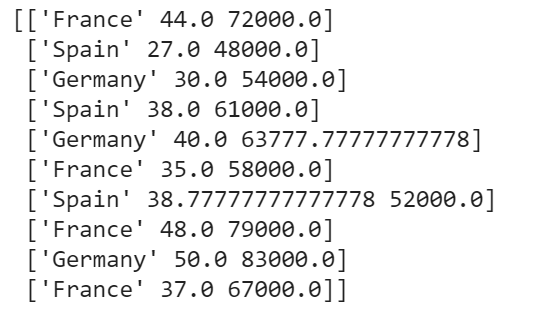
print(x)
Encoding Categorical Data
Since, most of the machine learning models are based on Mathematical equations and you can intuitively understand that it would cause some problem if we can keep the Categorical data in the equations because we would only want numbers in the equations. So, we need to encode the Categorical Variable.
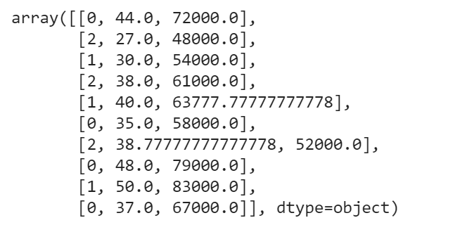
Like in our data set Country column will cause problem, so will convert into numerical values. To convert Categorical variable into Numerical data we can use *LabelEncoder() *class from preprocessing library.
from sklearn.preprocessing import LabelEncoder,OneHotEncoder
le_X = LabelEncoder()
x[:,0] = le_X.fit_transform(x[:,0])
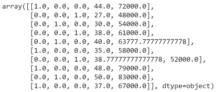
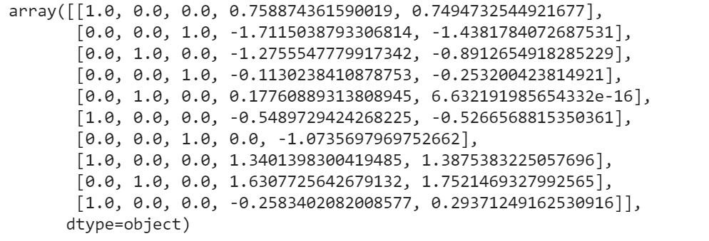
One-Hot Encoding One hot encoding takes a column that has categorical data and then splits the column into multiple columns. Depending on which column has what value, they are replaced by 1s and 0s.
In our example, we will get three new columns, one for each country — India, Germany, and Japan. For rows with the first column value as Germany, the ‘Germany’ column will be split into three columns such that, the first column will have ‘1’ and the other two columns will have ‘0’s. Similarly, for rows that have the first column value as India, the second column will have ‘1’ and the other two columns will have ‘0’s. And for rows that have the first column value as Japan, the third column will have ‘1’ and the other two columns will have ‘0’s.
➥ To implement One-Hot Encoding we need the help of the OneHotEncoder class of the scikit-learn libraries’ preprocessing module and the ColumnTransformer class of the compose module.
from sklearn.compose import ColumnTransformer
ct = ColumnTransformer([('encoder', OneHotEncoder(),[0])], remainder="passthrough") # The last arg ([0]) is the list of columns you want to transform in this step
x =np.array(ct.fit_transform(x))
x
Feature Scaling
Feature scaling is the method to limit the range of variables so that they can be compared on common grounds. See the Age and Salary column. You can easily noticed Salary and Age variable don’t have the same scale and this will cause some issue in your machine learning model.
Let’s say we take two values from Age and Salary column Age- 40 and 27 Salary- 72000 and 48000
One can easily compute and see that age column will be dominated. So, there are several ways of scaling your data.
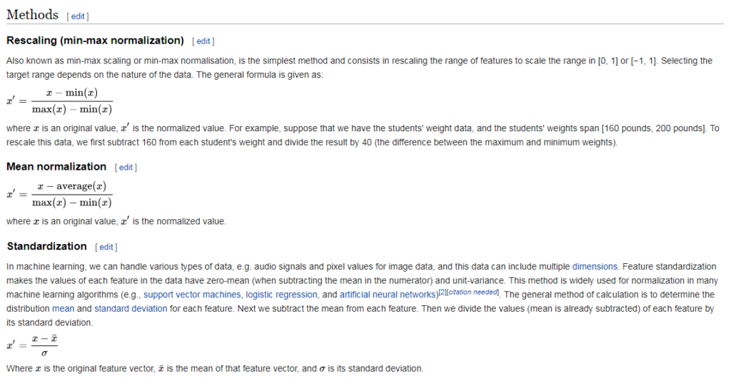
Since machine learning models rely on numbers to solve relations it is important to have similarly scaled data in a dataset. Scaling ensures that all data in a dataset falls in the same range.Unscaled data can cause inaccurate or false predictions.Some machine learning algorithms can handle feature scaling on its own and doesn’t require it explicitly.
As an example we give the code of the 3rd scalling method. We need to import the StandardScaler class of the scikit-learn library. Then we create the object of StandardScaler class. After that, we fit and transform the dataset
from sklearn.preprocessing import StandardScaler

sc = StandardScaler()

x[:, 3:] = sc.fit_transform(x[:, 3:])
x
Thanks for reading. If you like this, have a look at my other Data Science articles.
